
- << The ProofTools homepage
- >> The ProofTools manual page
- >> The feature comparison of free proof tree aka semantic tableau software
ProofTools background and technical addendum
Table of contents
- Introduction
- How proof trees work
- Breaking down a well-formed formula - the basics
- The disjunction rule
- The conjunction rule
- Example, step one: starting the tree
- Example, step two: applying the first disjunction rule
- Example, step three: applying the conjunction rule
- Simple well-formed formulas (simple wffs)
- Example, step four: applying the second disjunction rule
- Example, step five: applying the third disjunction rule
- Checking for closed branches
- The final tree: implications
- A note on necessary truth, logical truth and valuation
- Proof tree mechanics
- Checking arguments
- A clarification on validity and soundness, and contingent and necessary truth
- Breaking down a well-formed formula - the basics
- Proof tree rules
- Propositional logic proof tree rules
- The conjunction proof tree rule
- The negated conjunction proof tree rule
- The disjunction proof tree rule
- The negated disjunction proof tree rule
- The material conditional proof tree rule
- The negated material conditional proof tree rule
- The material equivalence proof tree rule
- The negated material equivalence proof tree rule
- The double negation proof tree rule
- Predicate logic proof tree rules
- Modal logic proof tree rules
- Propositional logic proof tree rules
- Logic operators
- Formation rules
- Left-to-right parsing versus right-to-left parsing
- Infinite branch detection
- Reference text
Introduction
This page provides background information and a technical addendum to the ProofTools manual. It is mostly concerned with explaining the concepts relevant to the ProofTools application: the basics of propositional, predicate and (to a much lesser extent) modal logic, and how and why proof trees work. If you don't know what it means for an argument to be valid or for a formula to be logically true, if you don't know what propositional, predicate or modal logic are, if you don't recognise the logical symbols used in the manual or the ProofTools software, or if you don't know what a proof tree is, then hopefully this page will help to inform you.
How proof trees work
ProofTools uses the proof tree method, also known as semantic tree, analytic tableau and semantic tableau, to check the validity of a logical proof, or to test the logical truth of a well-formed formula. Here is a brief introduction to the how and why of proof trees.
A proof tree is slightly unusual in that, to use it to check whether a well-formed formula is logically (i.e. necessarily or tautologically) true, the proof tree works not on the formula itself, but rather on the formula's negation. It breaks down the negation of the formula into a complete set of the different ways in which that negation of the formula could be true; each member of the set constitutes a branch of the proof tree. If a contradiction occurs on a branch, then the branch is said to "close", which is indicated with an asterisk. If all branches of the negation of the formula close, then it is impossible for that negation of the formula to be true, meaning that the original non-negated formula is a logical (necessary) truth - more on logical truths and necessity in the sections below, A note on necessary truth, logical truth and valuation and A clarification on validity and soundness, and contingent and necessary truth. The proof tree mechanism is also explained in more detail in the section below, Proof tree mechanics.
Breaking down a well-formed formula - the basics
The breaking down of a formula into a proof tree is best explained through example, so without further ado, here is an example proof tree. Our example is based on the propositional logic formula, ((A∨B)∧(¬A∨C))∨D. If you're not familiar with the symbols in that formula then you might want to read the section ahead, Propositional logic operators. The rest of this section will explain how we generate this proof tree from the original formula.
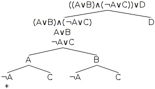
The tree is formed by applying rules to the nodes of the tree, starting with the first node (representing the original formula), until no more rules can be applied. Each node is labelled with a syntactically valid formula, also known as a well-formed formula (wff), as derived from the applied rule. To start with, and as pertains to this example tree, we will consider only two rules: the disjunction rule and the conjunction rule.
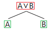
The disjunction rule
The disjunction rule specifies that if the top-level operator in a node's formula is a disjunction operator (i.e. ∨), then all branches below that node split into two nodes, with each of those two nodes being given a different one of the disjuncts (the disjunction operator's operands) as its formula.
This rule effectively splits that part of the tree below the node into the two ways in which it could be true: that of the first disjunct being true, and that of the second disjunct being true.
Note that there are other rules that also cause branch splits; these will be introduced later.
The conjunction rule
The conjunction rule specifies that if the top-level operator in a node's formula is a conjunction operator (i.e. ∧), then both conjuncts (the conjunction operator's operands) of that formula are added to all branches below it as new, consecutive, non-branching nodes.
This rule does not split the tree because both conjuncts must be true at the same time, which translates in terms of the proof tree into both conjuncts being true on the same branch.
Note that there are other rules that also cause non-branching nodes to be added; these will be introduced later.
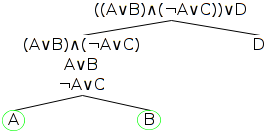
Example, step one: starting the tree
We start the tree with the original formula as the one and only node (newly added nodes will be circled in green in what follows). As explained above, when attempting to prove a formula to be logically true we will actually start with the negation of that formula, but for now we're less concerned about proof as we are about rule application, so whether the formula is negated or not is irrelevant.
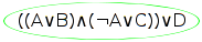
Example, step two: applying the first disjunction rule
Next, we examine the one and only node, and find that its top-level operator is the right-most disjunction operator, ∨. This operator operates on the disjuncts (A∨B)∧(¬A∨C) and D. Using the disjunction rule, then, we add both of these disjuncts as nodes to the branches of the tree below it (of which there is only one - the main branch). Thus we add the second and third nodes as (A∨B)∧(¬A∨C) and D, as shown circled below.
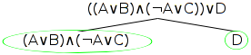
Next we take each of these new nodes in turn, and, if possible, apply a relevant rule to each one for all of the branches below it.
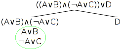
Example, step three: applying the conjunction rule
So, taking the first node, (A∨B)∧(¬A∨C), we note that the top-level operator is the conjunction operator, ∧, which operates on the two conjuncts A∨B and ¬A∨C. Using the conjunction rule, then, we add to the branch below that node two nodes, and label each node with one of the conjuncts - and so we add the fourth and fifth nodes as A∨B and ¬A∨C. Note that we don't add those two nodes to the branch to the right - the one ending in the node labelled D - because we only apply rules to branches below the node to which the rule is being applied.
Simple well-formed formulas (simple wffs)
Now we look at the next as-yet unexamined node in the tree, the one labelled D, and note that we cannot apply a rule to it because it does not contain any operators. It is a simple well-formed formula (simple wff). A simple wff has no operators, except optionally for a single preceding negation operator.
Example, step four: applying the second disjunction rule
Turning to the next as-yet unexamined node in the tree, the one labelled A∨B, we note that its only, and hence top-level, operator is a disjunction operator, ∨, with disjuncts A and B, and so we split the branch below it into two new nodes, A and B, as shown in the diagram below. Note again that we don't add those two nodes to the branch to the right - the one ending in the node labelled D - again because we only apply rules to branches below the node to which the rule is being applied.
Example, step five: applying the third disjunction rule
Turning to the next as-yet unexamined node in the tree, the one labelled ¬A∨C, we note that its only, and hence top-level, operator is also a disjunction operator, ∨, with disjuncts ¬A and C, and so we split both branches below it into two new nodes, ¬A and C, as shown in the diagram below. Once more note that we don't add those two nodes to the branch to the right - the one ending in the node labelled D - once again because we only apply rules to branches below the node to which the rule is being applied.
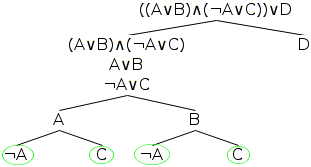
Noting that the remainder of the as-yet unexamined nodes in the tree are simple wffs, we find that we can't apply any more rules to the tree.
Checking for closed branches
Every time a rule is applied, we need to check each branch to which the rule added nodes to see whether it has closed. A branch is said to have closed when any two simple wffs along its path contradict one another, as, for example, the two simple wffs P and ¬P do. Taking our example, let's first identify the branches of the tree: there are five of them as indicated by the red, green, blue, cyan and orange coloured lines in the diagram below.
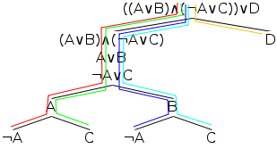
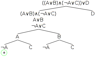
Now, checking up the red line of the first branch, we can see that two of its nodes containing simple wffs, the bottom-most node, ¬A, and the node second from the bottom, A, contradict one another. Thus, this branch has closed, and we mark it with an asterisk as shown in the diagram below.
The final tree: implications
Checking up the blue, green, cyan and orange lines of the remaining four branches, we find that we cannot identify any two contradictory simple wffs along any of those branches, so all of those branches remain open. All of the rules have been applied to the tree, and not all of the branches have closed, so the tree as a whole has not closed. We have therefore not proved that the negation of the first node's formula is necessarily true. Be careful, because this is not the same as proving that the negation of the first node's formula is necessarily false. This point is discussed in more detail towards the end of the section below, A clarification on validity and soundness, and contingent and necessary truth.
A note on necessary truth, logical truth and valuation
The following discussion includes references to the necessary or logical truth of well-formed formulas (wffs). Two points are worth noting in relation to this. The first is that some logicians hold that a wff cannot itself be true or false, but rather that it is only the valuation of that wff that can be true or false. Thus, rather than writing, "the necessary truth of the formula", they would write, "the necessary truth of the valuation of the formula". This document avoids that more unwieldy form and allows that a wff can itself be necessarily true.
The second point is a simple one: a formula that is necessarily true is also known as a logical truth, so in what follows, "logically true" and "necessarily true" are synonymous, as are "necessary truth" and "logical truth".
Proof tree mechanics
The fundamental mechanism of a proof tree is to detect contradictions. A contradiction in a formula entails that that formula is necessarily false, however, as was just pointed out, being free from contradiction does not entail being necessarily true, and thus a proof tree cannot be used to directly verify the logical truth of a given formula. Instead, a proof tree is used to test whether it is impossible for the negation of a formula to be true, which is the same as that negation of the formula being necessarily false, which is the same as the original (non-negated) formula being necessarily true.
The test for the impossibility of the negation of a formula being true is that described in the previous section: checking that all branches of the tree close, or in other words that all branches of the tree contain contradictions. Because the set of all branches represents all of the ways in which the tested negation of the formula could be true, then if all of them close (contain contradictions), the tested negation of the formula cannot be true, or is in other words necessarily false, meaning that the original (non-negated) formula is necessarily true. It's a slightly roundabout method of proving a formula's logical truth, but it's a reliable one.
Note that this description is intuitive; formal proofs of the soundness and completeness of the rules for proof trees can be found in the reference text by which ProofTools was developed.
Checking arguments
So far we've explained how a proof tree can determine whether an individual formula is a logical truth or not, but the introduction noted that ProofTools can validate entire arguments - so how do we go from checking whether an individual formula is a logical truth to checking whether an argument is valid? Thankfully, it's not very difficult.
An argument consists of a set of premises, each of which is a well-formed formula - let's call them P1, P2 and P3 - and a conclusion, also a well-formed formula - let's call it C. Now, testing the validity of the argument - i.e. whether the conclusion follows necessarily from the premises - is equivalent to testing whether the individual formula (P1∧P2∧P3)→C is a logical truth.
This formula can be converted into the logically equivalent formula, ¬(P1∧P2∧P3)∨C, which in turn can be converted using De Morgan's theorem into the logically equivalent formula, ¬((P1∧P2∧P3)∧¬C), from which we can remove the inner parentheses to arrive at ¬(P1∧P2∧P3∧¬C). So, to test the validity of the argument we simply - by virtue firstly of the fact that a proof tree tests the negation of a formula so that we can remove the preceding negation sign, and secondly of the conjunction rule - start off the tree as a single branch where each of the premises appears once as a node, and so does the conclusion, except that the conclusion is negated.
This is the structure that ProofTools works with, but it should be noted that, because it is negated, entering a conclusion alone is equivalent to testing the necessary truth of that formula (the entered conclusion) alone - in other words, premises are optional.
A clarification on validity and soundness, and contingent and necessary truth
What exactly do we mean when we say that a truth is a logical truth (a necessary or tautological truth), or that an argument is valid? - for these are exactly what ProofTools and proof trees in general test for. Validity and logical truth are essentially statements about the form and structure of formulas or arguments, and not about their content.
To say that a formula is logically true is to say that regardless of the truth of its components, and regardless of what those components represent, the formula will always be true by virtue of its form and structure - that it is impossible for it to be false, no matter whether the individual propositions and predicates (as symbolised in ProofTools by capital letters) in it are true or false, and no matter what the nature of those propositions and predicates is.
What it is not to say is that any or all of the individual propositions and predicates in the formula are true - any or all of these can be false and despite their being false the formula will remain (necessarily) true by virtue of its form and structure. This might seem to be an elementary point, but it's an important one to emphasise: don't confuse the overall necessary truth of a formula with the necessary truth of any of its components.
Similarly, to say that an argument is valid is to say that if its individual premises are true, then it is necessary that its conclusion is true - that it is impossible for the argument's conclusion to be false if its premises are all true.
What it is not to say is that any of those individual premises actually is true: unless a given premise is itself a necessary truth, then it might be false depending on what it represents, and what it represents is the input from "the real world". An argument is valid if its conclusion follows necessarily from its premises; an argument is sound if it is valid and if all of its premises actually are true.
Related to this is the fact that it is not necessary for an argument to be valid for its conclusion to be true: its conclusion could be accidentally or contingently true.
For an example of an accidentally true conclusion, first consider the following argument form which is invalid:
- P→A
- A
- Therefore P
Let's say that the propositions in this argument are such that in words, the argument is:
- Being a possum implies being an animal.
- This creature is an animal.
- Therefore this creature is a possum.
It's plain that the argument is invalid, and that therefore the conclusion is not necessarily true, but this is not to say that the conclusion cannot be true at all: unless it is necessarily false (which it isn't), then it could be accidentally or contingently true. Consider, for example, the possibility that the animal in question just happens to be a possum anyway: in this case even though the argument is invalid, the conclusion is true regardless.
Similarly, even if a formula is not necessarily/logically true (and to recap: it is necessary/logical truth which is tested for with ProofTools), then unless it is necessarily false (which can be tested for by testing the formula's negation in ProofTools), then it might anyway be contingently true. Consider as an example the formula M→H, which is not necessarily true, but not necessarily false either. This formula's truth is thus contingent on which propositions M and H represent. If we substitute propositions for M and H such that this formula in words is "Being a man implies being human", then it is in fact a true formula: being a man does imply being human. If, however, we substitute propositions for M and H such that this formula in words is "Being human implies being a man", then the formula is in fact false.
To summarise: just because a formula has been proved logically true, or an argument has been proved valid, by ProofTools or otherwise, does not mean that any of the individual components of the formula, or the premises of the argument, must be true. Also: just because a formula has not been proved logically true, or an argument has not been proved valid by ProofTools, does not mean that it or its conclusion (respectively) cannot anyway be true, unless the formula or the argument's conclusion (respectively) has been proved necessarily false: these can be done by testing in ProofTools the logical truth of the negation of the formula, or the validity of the argument's negated conclusion (respectively).
Proof tree rules
The diagrams for the rules assume that there are no other nodes below the node to which the rule is being applied, in other words that there is only one branch; if there are in fact multiple branches below the node (or, in the case of two-node rules, the node furtherest down the tree), then the new nodes indicated in the diagram need to be added to each of those branches, as demonstrated in the example above. Note, however, that ProofTools deals only with a single branch at a time, and postpones applications of rules to the other branches until the current branch either closes or can have no further rules applied to it - a note that could be repeated for each rule below but for readability will not be.
Each of these rules is only applicable when the relevant operator/s is/are the top-level operator/s; in what follows, A and B represent wffs, and are not necessarily individual propositions.
Propositional logic proof tree rules
Here follows a complete list of the propositional logic proof tree rules for all of the propositional logic operators supported by ProofTools.
Aside from the double negation rule, each of these rules can be derived by converting the operator expression into an equivalent expression in terms of conjunction and disjunction operators, and then applying the conjunction and disjunction rules to the resulting conversion. Those conversions are listed along with each operator.
The conjunction proof tree rule
The conjunction rule was explained earlier, in the example. From a conjunction (marked red) we append both conjuncts (marked green) to each branch below that conjunction.

The disjunction proof tree rule
The disjunction rule was explained earlier, in the example. From a disjunction (marked red) we split each branch below the disjunction in two, appending one of each of the disjuncts (marked green) to each side of the split.
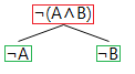
The negated conjunction proof tree rule
The formula for a negated conjunction, ¬(A∧B), is logically equivalent (per De Morgan's theorum) to the formula, ¬A∨¬B, and so the negated conjunction rule is based on the disjunction rule. Thus from a negated conjunction (marked red) we split each branch below it in two, appending one of each of the negated disjuncts (marked green) to each side of the split.
The negated disjunction proof tree rule
The formula for a negated disjunction, ¬(A∨B), is logically equivalent (per De Morgan's theorum) to the formula, ¬A∧¬B, and so the negated disjunction rule is based on the conjunction rule. Thus from a negated disjunction (marked red) we append both negated disjuncts (marked green) to each branch below that negated disjunction.

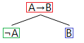
The material conditional proof tree rule
The formula for a material conditional, A→B, is logically equivalent to the formula, ¬A∨B, and so the material conditional rule is based on the disjunction rule. From a material conditional (marked red) we split each branch below it in two, appending to one side of each split the negated antecedent (marked green) and to the other side of the split the consequent (marked blue).
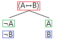
The negated material conditional proof tree rule
The formula for a negated material conditional, ¬(A→B), is logically equivalent to the formula, A∧¬B, and so the negated material conditional rule is based on the conjunction rule. From a negated material conditional (marked red) we append both the antecedent (marked green) and the negated consequent (marked blue) to each branch below that negated disjunction.

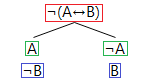
The material equivalence proof tree rule
The formula for a material equivalence, A↔B, is logically equivalent to the formula, (¬A∧¬B)∨(A∧B), and so the material equivalence rule is based on both the conjunction and disjunction rules. From a material equivalence (marked red) we split each branch below it in two, appending to one side of each split both the negated antecedent (marked green) and the negated consequent (marked blue), and to the other side of the split both the antecedent (marked green) and the consequent (marked blue).
The negated material equivalence proof tree rule
The formula for a negated material equivalence, ¬(A↔B), is logically equivalent to the formula, (A∧¬B)∨(¬A∧B), and so the material equivalence rule is based on both the conjunction and disjunction rules. From a material equivalence (marked red) we split each branch below it in two, appending to one side of each split both the antecedent (marked green) and the negated consequent (marked blue), and to the other side of the split both the negated antecedent (marked green) and the consequent (marked blue).
The double negation proof tree rule
For a double negation (marked red) we append the formula with the double negation removed (marked green) to each branch below that double negation.

Predicate logic proof tree rules
Here follows a complete list of the predicate logic proof tree rules for all of the predicate logic operators supported by ProofTools.
The universal quantifier proof tree rule
When the top-level operator of a node (marked red) is a universal quantifier, then if there is another node (marked blue) - on the branch (above or below, or even the universal quantifier node itself if it contains a constant), the universal-quantifier node - whose formula contains a constant, then a new node (marked green) is added to the branch; the new node duplicates the universal-quantifier node except that each instance of the variable that the universal quantifier quantifies over is replaced by the constant.
If the blue node does not exist - i.e. if there are no constants in any of the nodes on a given branch passing through a universal-quantifier node - then for each such branch we apply this rule as described except that instead of using a constant already on the branch (the missing blue node), we introduce a new constant that does not occur anywhere else on the tree (in versions prior to 0.4 beta, where constants were limited, when running short of constants, ProofTools may loosen this restriction such that the new constant must not occur anywhere else on the branch only) to act as the variable-instances replacement.
Note that this rule is applied to the universal-quantifier node for each constant that occurs on the branch either above or below (or identical with) the universal-quantifier node (and the new node is added only to that branch), and is reapplied each time a new constant appears on a branch below it (again, the new node is added only to that branch) except when an infinite branch is detected, in which case it is not reapplied.

The negated universal quantifier proof tree rule
When the top-level operators of a node (marked red) are a negation operator immediately followed by a universal quantifier, then a new node (marked green) that duplicates the original node but in which the universal quantifier has been replaced by an existential quantifier and the negation operator has been moved inside the quantifier is added to all branches below that node.

The existential quantifier proof tree rule
When the top-level operator of a node (marked red) is an existential quantifier, then a new node (marked green) is added to all branches below that node with all tokens of the variable that the existential quantifier quantifies over replaced by a constant that does not already appear on the tree.

The negated existential quantifier proof tree rule
When the top-level operators of a node (marked red) are a negation operator immediately followed by an existential quantifier, then a new node (marked green) which duplicates the original node but in which the existential quantifier has been replaced by a universal quantifier and the negation operator has been moved inside the quantifier is added to all branches below that node.

The Substitutivity of Identicals (SI) proof tree rule
When an identity node (marked red) is present on a branch, and also present on that branch is another node (marked blue) containing one or more instances of one the constants/variables of the identity node, then a new node (marked green) is added to each of the branches below these nodes, where one or more instances of the constant/variable in the second node is/are replaced with the other constant/variable from the identity node. This might be a little confusingly worded, so it might help to also quote from the reference text:
A is any atomic sentence distinct from a = b. (It could be any sentence, but this is enough, and makes for more manageable tableaux.)
SI says, in effect, that when we have a line of the form a = b we can substitute b for any number of occurrences of a in any line (above or below) with an atomic formula. Thus, suppose that the line is of the form Saa. This is (Sxa)x(a), (Sax)x(a), and (Sxx)x(a). Hence, we can apply the rule to get, respectively, (Sxa)x(b), (Sax)x(b), and (Sxx)x(b); that is, Sba, Sab, and Sbb.
This rule is not applied for a branch where to do so would result in a node duplicating one already present on the branch in question.

Modal logic proof tree rules
Here follows a complete list of the modal logic rules applied by ProofTools. Note that in modal logic trees, a world number is associated with each node. This number follows the node after a comma. Initial nodes have a world number of zero. When S5 is not active, novel types of nodes are possible: they take the form irj where i and j are world numbers. Intuitively, irj means "world i accesses world j". S5 trees skip these nodes, not because they no longer apply, but because they are redundant. For want of a known term, we will refer to these nodes as "world accessors".
The necessity proof tree rule
When the top-level operator of a node (marked red) is that of necessity, then (if S5 is not enabled) if there is a world accessor node (marked blue) whose LHS (left-hand side) world number matches that of the node, then a new node (marked green) identical to the original node except with the universal quantifier removed and the world number replaced by the world accessor's RHS (right-hand side) world number is added to all branches below it. If S5 is enabled, the new world number is taken from any other node's (marked blue) world number. To avoid repetition, this rule is not applied to any two given nodes on any given branch where to do so would result in a node duplicating one already present on that branch.
Note that this rule is applied to the necessity node for each world number that occurs on the branch either above or below the the necessity node (and the new node is added only to that branch), and is reapplied each time a new world accessor (if S5 is not enabled) or new node with new world number (if S5 is enabled) appears on a branch below it (again, the new node is added only to that branch) except when an infinite branch is detected, in which case it is not reapplied.
The negated necessity proof tree rule
When the top-level operators of a node (marked red) are a negation operator immediately followed by a necessity operator, then a new node (marked green) which duplicates the original node (including its world number) but in which the necessity operator has been replaced by a possibility operator and the negation operator has been shifted to the right is added to all branches below the node.

The possibility proof tree rule
When the top-level operator of a node (marked red) is that of possibility, then (if S5 is not enabled) two new nodes are added to each branch below it: the first (marked blue), a world accessor whose LHS world number is taken from the node and whose RHS world number is a new one not yet present on the branch, the second (marked green), identical to the original node except with its possibility operator removed and its world number replaced with the RHS world number of the added world accessor. If S5 is enabled, the first node is skipped and the new world number simply applied to the second (rather, in this case, the only, and also marked green) new node.

The negated possibility proof tree rule
When the top-level operators of a node (marked red) are a negation operator immediately followed by a possibility operator, then a new node (marked green) which duplicates the original node (including its world number) but in which the possibility operator has been replaced by a necessity operator and the negation operator has been shifted to the right is added to all branches below the node.

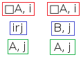
The modal reflexivity proof tree rule
This rule is not applied to S5 trees. Otherwise, when i is any world number present anywhere on a branch (i.e. in a node of a form marked red), including on the LHS or RHS of a world accessor, then a new world accessor node, iri (marked green), is added to the branch. This rule is not applied to a branch when to do so would result in a node duplicating one already present on that branch.
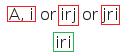
The modal symmetry proof tree rule
This rule is not applied to S5 trees. Otherwise, when a node (marked red) is a world accessor of the form irj, then a new world accessor node jri (marked green) is added to each branch below the given node. This rule is not applied to a branch when to do so would result in a node duplicating one already present on that branch.

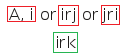
The modal transitivity proof tree rule
This rule is not applied to S5 trees. Otherwise, when world accessor nodes of the form irj (marked red) and jrk (marked blue) exist on the branch, then a new world accessor node irk (marked green) is added to each branch below the given nodes. As with the previous rules, this rule is not applied to a branch when to do so would result in a node duplicating one already present on that branch.

The modal extendability proof tree rule
When i is a world number in any node on a branch (i.e. in a node of a form marked red), then a new world accessor node irk (marked green), where k does not already appear on the branch, is added to that branch. The application of this rule is postponed until all other rules have been applied to the branch.
Logic operators
Propositional logic operators
The propositional logic operators supported by ProofTools, and their semantics, including truth tables, are as follows.
The conjunction operator, ∧
The conjunction operator, ∧, also known as "logical and", has the meaning implied by the everyday linguistic "and": its result is true only when both of its conjuncts are true.
| A | B | A∧B |
|---|---|---|
| False | False | False |
| False | True | False |
| True | False | False |
| True | True | True |
The disjunction operator, ∨
The disjunction operator, ∨, also known as "logical or", has the meaning implied by the everyday linguistic "or": its result is true when either of its disjuncts is true, with the clarification that its result is true when both of its disjuncts are true.
| A | B | A∨B |
|---|---|---|
| False | False | False |
| False | True | True |
| True | False | True |
| True | True | True |
The material conditional operator, →
The material conditional operator, →, arguably has the meaning implied by the everyday linguistic "if..then" construct, i.e. "If A then B". Formally, the semantics of the material conditional operator are stipulated such that if the antecedent is true, then the consequent must be true too, which covers the case of the antecedent being true; for a false antecedent the result of the material conditional operator is simply stipulated to be true.
| A | B | A→B |
|---|---|---|
| False | False | True |
| False | True | True |
| True | False | False |
| True | True | True |
The material equivalence operator, ↔
The semantics of the material equivalence operator, ↔, are stipulated such that it is true either if both the antecedent and the consequent are true, or if both the antecedent and the consequent are false; otherwise it is false.
| A | B | A↔B |
|---|---|---|
| False | False | True |
| False | True | False |
| True | False | False |
| True | True | True |
The negation operator, ¬
The negation operator, ¬, also known as "not", has the meaning implied by the everday linguistic "not": it reverses the truth value of that to which it is applied.
| A | ¬A |
|---|---|
| False | True |
| True | False |
Predicate logic operators
Quantification operators (∀ and ∃)
The two predicate logic quantification operators, the universal quantifier, ∀, and the existential operator, ∃, are used to quantify a variable in a predicate. A complete description of predicate logic is beyond the scope of this page: instead, a few examples will be provided to give a sense of what these operators mean.
To explain the universal quantifier, take for example the well-formed formula, ∀xRxc. Given an appropriate interpretation of Rxc as meaning "Person x recognises person c", this formula might be translated into English (where the symbols in the formula from which the preceding words were derived are parenthesised) as, "For all (∀) persons (x) it is the case that those persons (x) recognise (R) one person in particular (c)." In everyday language, this could be expressed as, "Everybody recognises person c."
To explain the existential quantifier, let's take that same example and simply change the quantifier, so that it now reads, ∃xRxc. Given the same interpretation of Rxc as previously, this formula might be translated into English as, "There exists (∃) a person (x) such that it is the case that that person (x) recognises (R) one person in particular (c)." In everyday language, this could be expressed as, "Somebody recognises person c."
Identity (=) and negated identity (≠)
The semantics of these operators are intuitive: they express that the constant/variable on the left hand side of the operator is or is not (respectively) identical with that on the right, meaning that whatever entity the one represents, the other does / does not also represent it.
Modal logic operators
The two modal logic operators are the necessity operator, □, and the possibility operator, ◊. Intuitively, □ can be read as "It is necessarily the case that", and ◊ can be read as "It is possibly the case that". Modal logic can be thought of in terms of possible worlds and the relations between them. Different stipulated relation constraints (i.e. reflexivity, symmetry, transitivity and extendability) result in different modal logics. A complete description of the modal logics supported by ProofTools (all are normal modal logics with constant domain and contingent identity) is beyond the scope of this page, however they are fully described in chapters 2, 3, 14 and 17 of our reference text.
Formation rules
This section defines well-formed formulas (wffs) as recognised by ProofTools (default syntax; Tarski's world syntax has some variations); the definition is recursive.
Note, however, that these formation rules do not take account of ProofTools's tolerance for extraneous whitespace, which can occur anywhere in any amount except within predicate/proposition/constant/variable names, where it is forbidden.
Formation rules for propositional logic
The formation rules for propositional logic wffs as recognised by ProofTools are as follows:
- Any single capital letter optionally followed by any number of digits is a wff.
- If A is a wff, then so is ¬A.
- If A and B are wffs, then so are A∧B, A∨B, A→B and A↔B.
- If A is a wff, then so is (A).
Suppose, for example, that we want to prove that (P∧Q)→P is a wff. We can do this by finding a way to build it in steps using the rules above:
| 1. P | [rule 1] |
| 2. Q | [rule 1] |
| 3. P∧Q | [rule 3 applied to lines 1 and 2] |
| 4. (P∧Q) | [rule 4 applied to line 3] |
| 5. (P∧Q)→P | [rule 3 applied to lines 4 and 1] |
Formation rules for predicate logic
The formation rules for predicate logic wffs as recognised by ProofTools are as for propositional logic, with these additions (remembering that a predicate name is defined in ProofTools as a single capital letter, optionally followed by any number of digits, a constant is defined as a single lowercase letter a through v minus t, optionally followed by any number of digits, and that a variable is defined as a single lowercase letter w through z plus t, optionally followed by one or more digits):
- Any predicate name followed by n constants (those constants can be the same or different) is a wff.
- If a and b are constants, then a=b and a≠b are wffs.
- If A is a wff containing at least one constant in which all occurrences of any particular constant have been replaced by a variable (for example, x), then (using x as an example) ∀xA and ∃xA are wffs.
- If ∀xA is a wff, then so are (∀x)A, ((∀x))A, (((∀x)))A, etc. Likewise, if ∃xA is a wff, then so are (∃x)A, ((∃x))A, (((∃x)))A, etc. (All of these are included for maximal flexibility in input, and are interpreted by ProofTools in the same way as without parentheses).
Suppose, for example, that we want to prove that ∀x∃y¬Rxy is a wff. We can do this by finding a way to build it in steps using the rules above:
| 1. Rab | [rule 5] |
| 2. ¬Rab | [rule 2 on line 1] |
| 3. ∃y¬Ray | [rule 7 on line 2 choosing constant b, variable y and quantifier ∃] |
| 4. ∀x∃y¬Rxy | [rule 7 on line 3 choosing constant a, variable x and quantifier ∀] |
Here is another example, proving that ∀xFx→∃xFx is a wff:
| 1. Fa | [rule 5] |
| 2. ∀xFx | [rule 7 on line 1 choosing constant a, variable x and quantifier ∀] |
| 3. ∃xFx | [rule 7 on line 1 choosing constant a, variable x and quantifier ∃] |
| 4. ∀xFx→∃xFx | [rule 3 on lines 2 and 3] |
Formation rules for modal logic
The formation rules for modal logic wffs as recognised by ProofTools are as for predicate logic, with this addition:
- If A is a wff, then so are □A and ◊A.
Left-to-right parsing versus right-to-left parsing
In the ProofTools manual it is noted that for all operators other than material conditional, parsing a pair of the same operator, unparenthesised, from left-to-right is identical with parsing that same formula from right-to-left, and here we present the proof trees to demonstrate that.
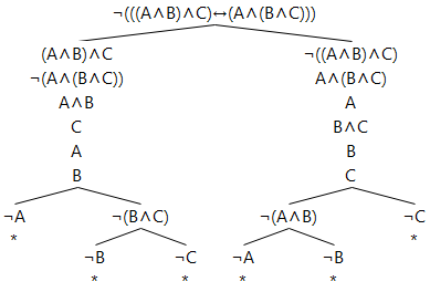
The equivalence of left-to-right parsing and right-to-left parsing for conjunction
This proof tree proves that parsing the formula A∧B∧C left-to-right as (A∧B)∧C is identical with parsing it right-to-left as A∧(B∧C):
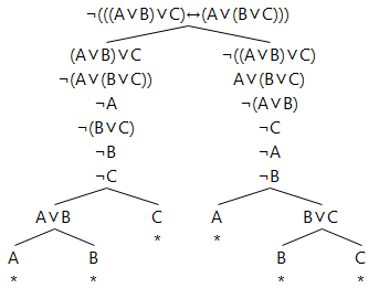
The equivalence of left-to-right parsing and right-to-left parsing for disjunction
This proof tree proves that parsing the formula A∨B∨C left-to-right as (A∨B)∨C is identical with parsing it right-to-left as A∨(B∨C):
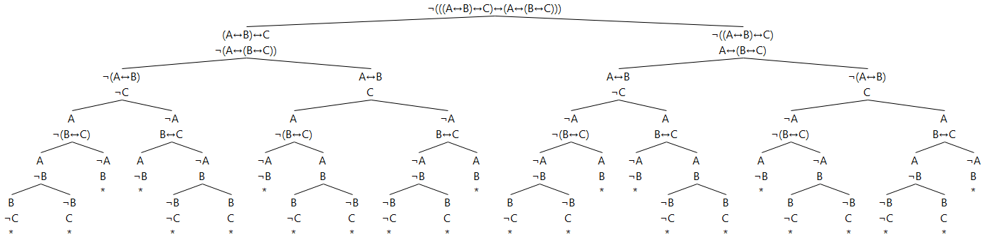
The equivalence of left-to-right parsing and right-to-left parsing for material equivalence
This proof tree (click on it for the full size image if it is shrunken in your browser) proves that parsing the formula A↔B↔C left-to-right as (A↔B)↔C is identical with parsing it right-to-left as A↔(B↔C):
Infinite branch detection
Note well: Infinite branch detection has been disabled from version 0.6 aside from straightforward detection of infinite branches due to application of the modal extensibility rule. This is because the algorithm (below) is flawed and gives the wrong results in some cases. Because predicate logic is undecidable, there can be no perfect algorithm for detecting infinite loops. Thus, in some way, the following algorithm is necessarily incorrect. Too, we have found at least one case in which it definitively fails. You can read more about this bug in the update of 2019-02-09. Other than this note, I have left this section unchanged from when we believed the algorithm to be functional.
Infinite loops are possible under certain conditions under the predicate and modal logic proof tree rules as listed above and as used by ProofTools. These conditions are, specifically:
- When at least one node occurs in the tree in which an existential quantifier falls within the scope of a universal quantifier.
- Under certain combinations of reflexivity (ρ), symmetry (σ) and transitivity (τ) - in particular, S5 - when at least one node occurs in the tree in which a possibility operator falls within the scope of a necessity operator, and when that outer necessity operator has the possibility rule applied to it at least once for some reason (e.g. because it in turn falls within the scope of an outer possibility operator, or because there is another node in the tree whose outer operator is possibility).
- When extendability (η) is enabled and the tree does not close even after postponing the application of the extendability rule until no other rules are pending.
The simplest example demonstrating such an infinite loop under the first condition is the proof tree broken down from the well-formed formula, ∀x∃yPxy. The proof tree for this well-formed formula breaks down as follows:
| ∀x∃yPxy | [first node] |
| ∃yPay | [universal quantifier rule on first node] |
| Pab | [existential quantifier rule on second node] |
| ∃yPby | [universal quantifier rule on first and third nodes] |
| Pbc | [existential quantifier rule on fourth node] |
| ∃yPcy | [universal quantifier rule on first and fifth nodes] |
| Pcd | [existential quantifier rule on sixth node] |
| ∃yPdy | [universal quantifier rule on first and seventh nodes] |
| Pde | [existential quantifier rule on eighth node] |
| ∃yPey | [universal quantifier rule on first and nineth nodes] |
| Pef | [existential quantifier rule on tenth node] |
| etc... |
Infinite loops can be detected and prevented in general under the first two conditions by following these rules, which is conceptually how ProofTools does it (note that it might be easier to read what follows on the understanding that the systems for detecting universal node-based infinite loops and for detecting necessity node-based infinite loops are separate and essentially identical in procedure; they are described together because they are so similar: it might help to read what follows by focussing on only one of the systems at a time):
- Number consecutively each node whose top-level operator is a universal quantifier / necessity operator. Separate sequences of numbers are used for each of these two types of operators - call each of these numbers, respectively the "ancestral universal node number" and the "ancestral necessity node number" i.e. the first universal quantifier node has an ancestral universal node number of 1, and the first necessity operator node has an ancestral necessity node number of 1; whilst the value of the number is the same in each case, its association (with either universal quantifier nodes or with necessity operator nodes) is different.
- Associate with each node two lists, one of ancestral universal node numbers and the other of ancestral necessity node numbers. Call the first list the "ancestral universal nodes list", and the second, the "ancestral necessity nodes list".
- The lists of all of the initial nodes on the tree are empty.
- Each node, N, inherits both the ancestral universal nodes list and the ancestral necessity nodes list of the node to which a rule was applied to generate that node N. In the case of a rule application in which a second node - e.g. the one containing the constant in a universal rule application, or any of the modal rules involving two nodes - exists, then the generated node N inherits as its ancestral universal node list the combined ancestral universal node lists of both nodes used to generate it, and likewise for its ancestral necessity node list: it inherits the combined lists of both nodes used to generate it.
- In addition, and which is how the lists are initially populated, any node generated using the universal quantifier rule has appended to its ancestral universal nodes list the ancestral universal node number of the universal quantifier node from which it was generated, and any node generated using the necessity rule has appended to its ancestral necessity nodes list the ancestral necessity node number of the necessity node from which it was generated.
Now, an infinite loop can be detected under the first condition by checking for any potential universal rule application whether the ancestral universal node number of the universal-quantifier node to which the potential rule would be applied occurs within the ancestral universal nodes list of the node containing the constant which per the potential rule application would replace the variable of the universal quantifier. If the node number does occur in the list, then an infinite loop will inevitably ensue, and it can be avoided by refraining from applying the rule - and so ProofTools refrains.
Likewise, an infinite loop can be detected under the second condition by checking for any potential necessity rule application whether the ancestral necessity node number of the necessity-operator node to which the potential rule would be applied occurs within the ancestral necessity nodes list of the node containing the world number which per the potential rule application would replace the world number of the formula to which the necessity operator applies. If the node number does occur in the list, then an infinite loop will inevitably ensue, and it can be avoided by refraining from applying the rule - and so ProofTools refrains.
Infinite loops can be detected and prevented under the third condition by following this rule: apply any (potential) extendability rule only when there are no other rules to apply. If the extendability rule has already been applied, and since applying it no other rules other than world accessors have been applied, then an infinite loop will inevitably ensue, and it can be avoided by refraining from applying the rule - and so ProofTools refrains.
A rigorous proof that these rules are sufficient, minimal and correct in preventing and detecting infinite loops - i.e. that they detect every infinite loop, and that they do not falsely detect infinite loops and/or prevent trees that can be closed from closing - is, for the moment, beyond the author's patience. If, however, you become aware of any situation in which they fail, then I would very much like to know.
Reference text
The reference text in the development of ProofTools has been, and continues to be, Graham Priest's An Introduction to Non-Classical Logic, Second Edition, published by Cambridge University Press in 2008 (with a third printing in 2010), ISBN 978-0-521-67026-5 (paperback) and ISBN 978-0-521-85433-7 (hardback).
